
Datasets, Graph Representations, and Inference Mechanics
Graph Neural Networks (GNNs) extend traditional deep learning models to graph-structured data G = (V, E) consisting of vertices V and edges E. Unlike standard vector or grid-based inputs, real-world estimation tasks frequently rely on graph structures where individual data points are interconnected by relationships.
1. Real-World Graph Datasets
The Cora Dataset
The Cora dataset represents a citation network designed for node classification tasks:
- Network Structure: Consists of 2,708 scientific publications linked together by 5,429 undirected citation edges.
- Node Features: Each publication is represented by a binary word feature vector of length 1,433, where each entry denotes the presence (1) or absence (0) of a unique dictionary word.
- Task Objective: Predict the broad subject category of each paper across seven distinct classes.
| Subject Category | Publication Count |
| Neural_Networks | 818 |
| Probabilistic_Methods | 426 |
| Genetic_Algorithms | 418 |
| Theory | 351 |
| Case_Based | 298 |
| Reinforcement_Learning | 217 |
| Rule_Learning | 180 |
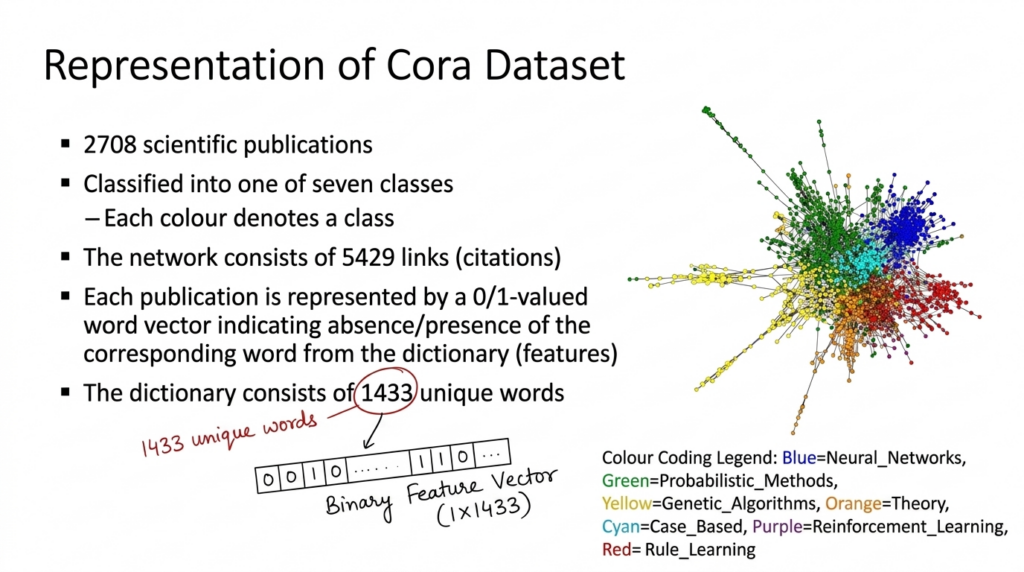
In visual graph representations of Cora, seven distinct colors highlight how papers cluster structurally based on their subject domains.
The REDDIT-Binary Dataset
The REDDIT-Binary benchmark models dynamic online user interactions on Reddit:
- Graph Definition: Nodes represent individual Reddit users, while an edge connects two users if at least one user responded to the other’s comment.
- Classification Level: Performs graph-level binary classification to determine whether an online community is Question/Answer-based or Discussion-based.
- Scale: Contains 232,965 nodes, 114,615,892 edges, and a feature vector length of 602 per node.
2. Graph Representation & Matrix Formulations
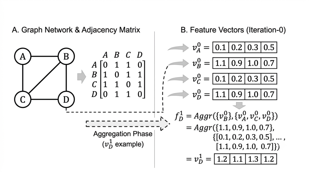
A graph is represented algebraically by its Adjacency Matrix A in \{0, 1\}^{\vert{}V\vert{} \times \vert{}V\vert{}}$ alongside per-node feature vectors. For an unweighted 4-node system (A, B, C, D), an entry A_{ij} = 1 indicates a direct connection between node i and node j:
A = | 0 1 1 1 |
    | 1 0 1 0 |
    | 1 1 0 0 |
    | 1 0 0 0 |
Each node maintains an initial feature vector f_1:
- Node D: f_1^D = [1.1, 0.9, 1.0, 0.7]
- Node A: f_1^A = [0.1, 0.2, 0.3, 0.5]
3. GNN Inference Mechanics
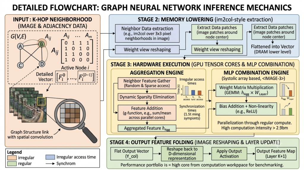
GNN inference operates over multiple iterative steps. Each iteration consists of two sequential operations: Aggregation and Combination.
┌────────────────────────┐      ┌────────────────────────┐      ┌────────────────────────┐
│  Neighborhood Feature  │ ───► │   Aggregation Phase    │ ───► │CombinationPhase    │
│  Collection (f_A, f_D) │      │   g(f_1^D, f_1^A)      │      │     (Shallow MLP)      │
└────────────────────────┘      └────────────────────────┘      └────────────────────────┘
                                                                            │
                                                                            ▼
                                                                ┌────────────────────────┐
                                                                │  Next Iteration Input  │
                                                                │ [0.73, 0.68, 0.13]     │
                                                                └────────────────────────┘
Step 1: Aggregation
In the aggregation step, a node collects feature vectors from all its immediate neighbors as well as its own state. An aggregation function g(.) (such as element-wise addition) synthesizes these vectors into an intermediate feature vector f_D:
f_D = g(f_1^D, f_1^A) = f_1^D + f_1^A = [1.2, 1.1, 1.3, 1.2]
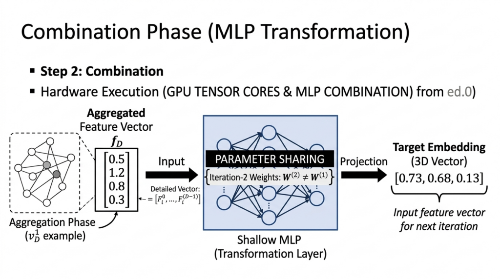
Step 2: Combination
In the combination step, the aggregated feature vector f_D is fed into a shallow Multi-Layer Perceptron (MLP). The MLP transforms the input into a new target embedding space (e.g., mapping a 4-dimensional aggregated vector into a 3-dimensional output vector [0.73, 0.68, 0.13]). This output becomes the input feature vector for the next iteration.
4. Fundamental Architectural Rules
Two structural properties characterize standard message-passing Graph Neural Networks:
- Parameter Sharing Across Nodes: Within a single iteration, all nodes across the entire graph share the exact same MLP structure and weight values.
- Layer-Wise Independence: Each iteration utilizes a distinct, separate MLP network.