
Unifying Convolutions and GEMM
Deep learning frameworks like PyTorch and TensorFlow provide an operational abstraction that allows researchers to design neural networks using geometric intuition. A convolutional layer is typically visualized as a 3D filter sliding across a spatial grid. While this geometric mental model is mathematically accurate for theoretical design, it is computationally disastrous if implemented directly on bare-metal silicon.
To achieve the sub-millisecond execution speeds required for production inference and massive distributed training, compilers and hardware backends (like NVIDIA cuDNN) must shatter this spatial illusion. They perform computational lowering: the process of translating high-level spatial operations into highly optimized, low-level linear algebra routines.
1. The 7-Loop Fallacy and Hardware Inefficiency
The naive implementation of a 2D batch convolution over a 4D tensor input requires an execution pipeline nested seven levels deep. Given a batch of images $N$, input channels $C_{in}$, spatial dimensions $H \times W$, and a filter $K_H \times K_W$, the standard spatial convolution evaluates to:
Python
# The Naive 7-Loop Convolution
for n in range(N):
    for co in range(C_out):
        for ho in range(H_out):
            for wo in range(W_out):
                for ci in range(C_in):
                    for kh in range(K_H):
                        for kw in range(K_W):
                            # Sequential memory access and arithmetic
                            Y[n, co, ho, wo] += X[n, ci, ho*stride+kh, wo*stride+kw] * W[co, ci, kh, kw]
From a systems engineering perspective, this algorithm is hostile to modern hardware.
- Cache Thrashing: The nested strides and non-contiguous memory access patterns cause severe L1 and L2 cache misses on the GPU.
- SIMD Underutilization: Single Instruction, Multiple Data (SIMD) vector units and hardware Tensor Cores are designed to execute massive block-matrix multiply-accumulate (MAC) operations simultaneously. The 7-loop structure forces sequential, scalar-like execution pipelines that leave over 90% of a GPU’s floating-point units idle.
2. Matrix Unrolling via im2col
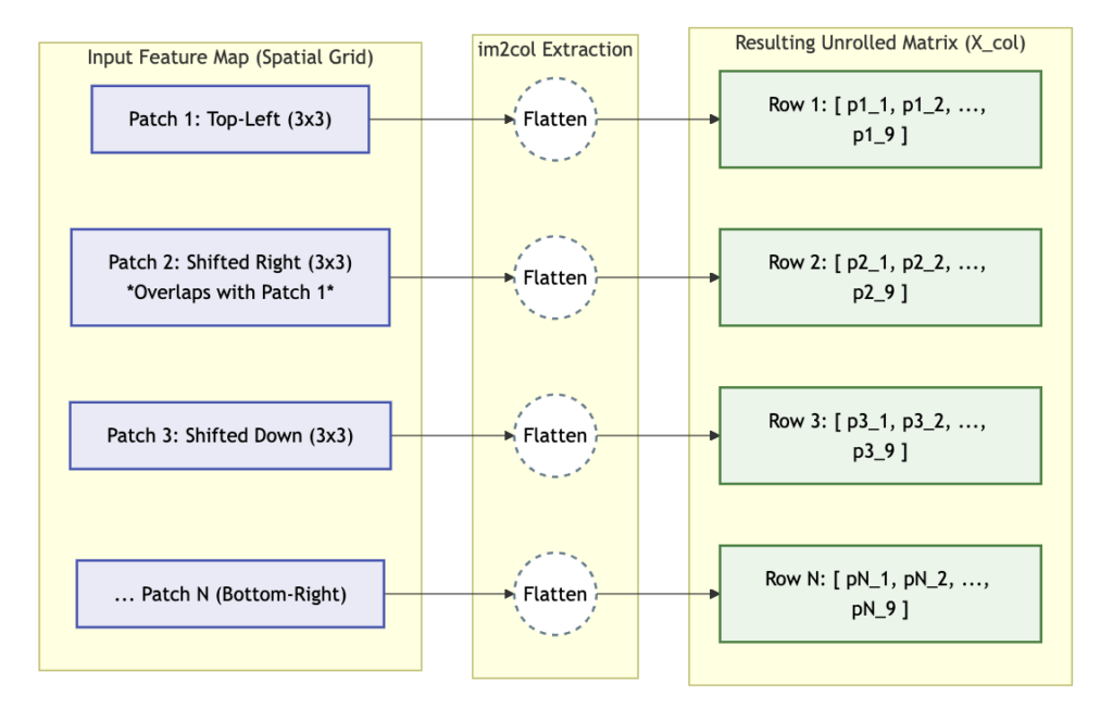
To bypass the inefficiency of nested loops, low-level execution engines transform the multi-dimensional sliding window problem into a flat, 2D matrix multiplication problem. This relies on an algorithmic transformation known as im2col (Image to Column).
The goal of im2col is to extract every localized spatial patch that a convolutional kernel will touch and flatten it into a single column (or row) of a massive 2D matrix.

Let the input tensor be $X \in \mathbb{R}^{N \times C_{in} \times H \times W}$. For a given stride and padding, the output spatial dimensions are $H_{out}$ and $W_{out}$. The im2col algorithm extracts patches of size $C_{in} \times K_H \times K_W$ and flattens each into a vector of length $C_{in} \cdot K_H \cdot K_W$.
Since there are $H_{out} \cdot W_{out}$ such patches per image, and $N$ images in the batch, the resulting unrolled input matrix $X_{col}$ takes the exact shape:
$$X_{col} \in \mathbb{R}^{(N \cdot H_{out} \cdot W_{out}) \times (C_{in} \cdot K_H \cdot K_W)}$$
Simultaneously, the 4D weight tensor $W \in \mathbb{R}^{C_{out} \times C_{in} \times K_H \times K_W}$ is statically reshaped (without memory duplication) into a 2D matrix $W_{row}$:
$$W_{row} \in \mathbb{R}^{C_{out} \times (C_{in} \cdot K_H \cdot K_W)}$$
The Memory Trade-off: The im2col transformation involves significant memory duplication. Because convolutional patches overlap, the same input pixels are copied multiple times into different rows of $X_{col}$. This increases the memory footprint footprint substantially, trading VRAM capacity for pure computational throughput.
3. General Matrix Multiplication (GEMM) Execution
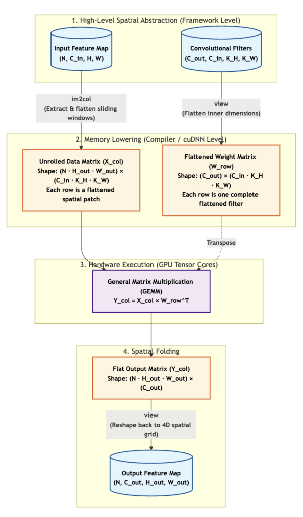
Once the input tensor and the weights are flattened into 2D matrices, the 7-loop convolution is reduced to a single, hyper-optimized General Matrix Multiplication (GEMM) call.
The output $Y_{col}$ is simply the matrix product of $X_{col}$ and the transposed weight matrix:
$$Y_{col} = X_{col} W_{row}^T$$
By inspecting the inner dimensions:
$$[(N \cdot H_{out} \cdot W_{out}) \times (C_{in} \cdot K_H \cdot K_W)] \times [(C_{in} \cdot K_H \cdot K_W) \times C_{out}]$$
The dot product collapses the shared dimension, yielding an output matrix:
$$Y_{col} \in \mathbb{R}^{(N \cdot H_{out} \cdot W_{out}) \times C_{out}}$$
This 2D matrix is then natively reshaped back into the expected 4D output tensor $Y \in \mathbb{R}^{N \times C_{out} \times H_{out} \times W_{out}}$. By converting the operation to GEMM, the GPU can tile the matrices into shared memory blocks and feed them directly into Tensor Cores, yielding the 5x to 20x speedups seen in modern deep learning compared to naive implementations.
4. The Unified Architectural Algebra
Stripping away the spatial abstraction reveals a profound mathematical reality about neural network architectures: Dense (Fully Connected) layers and Convolutional layers are computationally isomorphic.
Consider a standard Fully Connected (FC) layer applied to a flattened image. The input $X \in \mathbb{R}^{C_{in} \times H \times W}$ is flattened to a vector $x \in \mathbb{R}^{C_{in} \cdot H \cdot W}$. The Dense weight matrix $W_{dense}$ has the shape $C_{out} \times (C_{in} \cdot H \cdot W)$.
Now, consider a Convolutional layer where the kernel dimensions are intentionally set to match the exact spatial dimensions of the input feature map: $K_H = H$ and $K_W = W$.
Because the kernel covers the entire image in a single placement, the output spatial dimensions drop to $1 \times 1$. The 4D convolutional weight tensor has the shape $C_{out} \times C_{in} \times H \times W$.
When this convolution is lowered via im2col, the kernel flattening yields a 2D matrix of shape $C_{out} \times (C_{in} \cdot H \cdot W)$. The input matrix $X_{col}$ yields shape $1 \times (C_{in} \cdot H \cdot W)$. The resulting GEMM operation is perfectly identical to the Dense layer’s vector-matrix multiplication.
This mathematical proof—that a Dense layer is merely a Convolutional layer with a global kernel size—is the architectural foundation behind Fully Convolutional Networks (FCNs) like U-Net and YOLO, allowing models to accept dynamically sized input resolutions at inference time without breaking dimensional constraints.
5. End-to-End im2col Implementation in PyTorch
To solidify the lowering mechanics, this implementation manually extracts the sliding windows using PyTorch’s low-level unfold primitive (the PyTorch equivalent of im2col), performs the GEMM operation, and folds the tensor back into its spatial dimensions.
Python
import torch
import torch.nn.functional as F
import time

def manual_im2col_conv(x, weights, bias, stride=1, padding=0):
    """
    Executes a 2D convolution by manually lowering the tensors into
    2D matrices and routing them through a standard GEMM operation.
    """
    N, C_in, H, W = x.shape
    C_out, _, K_H, K_W = weights.shape

    # 1. Calculate output spatial dimensions
    H_out = (H + 2 * padding - K_H) // stride + 1
    W_out = (W + 2 * padding - K_W) // stride + 1

    # 2. im2col transformation: Extract sliding local blocks
    # unfold extracts patches and flattens the spatial dimensions
    x_unfolded = F.unfold(x, kernel_size=(K_H, K_W), padding=padding, stride=stride)

    # x_unfolded shape is currently: (N, C_in * K_H * K_W, H_out * W_out)
    # We transpose it to match our X_col mathematical derivation:
    # New shape: (N, H_out * W_out, C_in * K_H * K_W)
    X_col = x_unfolded.transpose(1, 2)

    # 3. Flatten weights into W_row
    # Shape becomes: (C_out, C_in * K_H * K_W)
    W_row = weights.view(C_out, -1)

    # 4. Execute GEMM
    # X_col (N, L, K) @ W_row.T (K, C_out) -> (N, L, C_out)
    Y_col = torch.matmul(X_col, W_row.t())

    # Add bias via broadcasting
    if bias is not None:
        Y_col += bias

    # 5. Reshape back to 4D spatial tensor
    # Transpose back to (N, C_out, H_out * W_out) and view as (N, C_out, H_out, W_out)
    Y_spatial = Y_col.transpose(1, 2).view(N, C_out, H_out, W_out)

    return Y_spatial

# --- Execution & Verification ---

# Define dimensions
N, C_in, H, W = 32, 64, 56, 56
C_out, K_H, K_W = 128, 3, 3
stride, padding = 1, 1

# Initialize random tensors
x = torch.randn(N, C_in, H, W)
weights = torch.randn(C_out, C_in, K_H, K_W)
bias = torch.randn(C_out)

# Run standard PyTorch C++ Backend Convolution
out_native = F.conv2d(x, weights, bias, stride=stride, padding=padding)

# Run our manual im2col + GEMM lowering
out_manual = manual_im2col_conv(x, weights, bias, stride=stride, padding=padding)

# Verify mathematical equivalence
max_diff = torch.max(torch.abs(out_native - out_manual))
print(f"Maximum discrepancy between Native and im2col GEMM: {max_diff.item():.6e}")
# Expected output: A value near 1e-5 or lower, verifying floating-point isomorphism.